

The Iris dataset is often used in machine learning and data science courses, because it’s simple to understand and well-defined, yet interesting enough to present real challenges to new learners. This tutorial will use Python to classify the Iris dataset into one of three flower species: Setosa, Versicolor, or Virginica.
What is the Iris dataset?
The iris data consisted of 150 samples of three species of Iris. The first column represented sepal length, the second column represented sepal width, the third column represented petal length, and the fourth column represented petal width. I'm going to use sci-kit-learn to classify these instances according to their species of Iris, which will be distinguished based on their measurements. The picture of the Iris species is given below:

In fact, three of these iris species look similar, but the difference in measurements can be used to classify them. This data set is a classic example of supervised learning. The input variables are sepal length and width and petal length and width; each row represents an instance or observation. The output variable is Iris-setosa, Iris-versicolor, or Iris-virginica; each column represents a class label.
Exploring the dataset
First, we need to import the dataset from the Scikit-learn library, or else you can find structured datasets from platforms like Kaggle. But for now, we are using the Iris dataset prebuilt on Scikit-learn.
from sklearn import datasetsimport pandas as pdimport numpy as npiris = datasets.load_iris() #Loading the datasetiris.keys()dict_keys(['data', 'target', 'frame', 'target_names', 'DESCR', 'feature_names', 'filename', 'data_module'])
The dataset contains some keys, which we can use to access specific data. For example, if we want to get the data about the length and width of Iris flowers, you can specify iris['data'].
Converting the dataset to pandas dataframe
Well, we have the data in our hands but it's not well structured for us to understand. So we need to convert it into a pandas DataFrame. Pandas is a great tool for doing all sorts of things related to datasets, including preprocessing and exploring them. So let's convert our dataset that is in the form of matrices into the form of rows and columns.
iris = pd.DataFrame(data= np.c_[iris['data'], iris['target']],columns= iris['feature_names'] + ['target'])
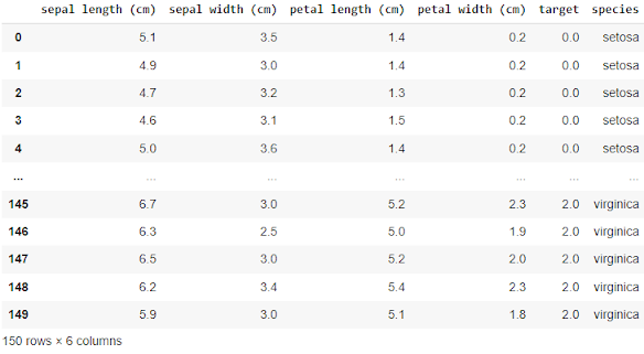
Now we will be using Pandas' built-in function 'head()' to see the first few rows of our data frame.
iris.head(10)sepal length (cm) sepal width (cm) petal length (cm) petal width (cm) target0 5.1 3.5 1.4 0.2 0.01 4.9 3.0 1.4 0.2 0.02 4.7 3.2 1.3 0.2 0.03 4.6 3.1 1.5 0.2 0.04 5.0 3.6 1.4 0.2 0.05 5.4 3.9 1.7 0.4 0.06 4.6 3.4 1.4 0.3 0.07 5.0 3.4 1.5 0.2 0.08 4.4 2.9 1.4 0.2 0.09 4.9 3.1 1.5 0.1 0.0
Here you can see that the iris data frame contains the length and width of sepals and petals including the target column which is the numerical representation of classes of Iris flowers that we need to classify (eg: Setosa(0), Versicolor(1), Virginica(2) ).
Since there is no column of names of species in the data frame let's add one more column with names of different species corresponding to their numerical values. It really helps us to access the different classes using their names instead of numbers.
species = []for i in range(len(iris['target'])):if iris['target'][i] == 0:species.append("setosa")elif iris['target'][i] == 1:species.append('versicolor')else:species.append('virginica')iris['species'] = species
This code will create another column in the data frame with names of different species.
 |
| iris data frame |
iris.groupby('species').size()speciessetosa 50versicolor 50virganica 50dtype: int64
Each number of classes has 50 instances together constituting 150 in total. You can also get some simple statistical information about the dataset by the "describe" method:
iris.describe()

Plotting the dataset
Plotting a dataset is a great way to explore its distribution. Plotting the iris dataset can be done using matplotlib, a Python library for 2D plotting.
The following code will plot the iris dataset,
import matplotlib.pyplot as pltsetosa = iris[iris.species == "setosa"]versicolor = iris[iris.species=='versicolor']virginica = iris[iris.species=='virginica']fig, ax = plt.subplots()fig.set_size_inches(13, 7) # adjusting the length and width of plot# lables and scatter pointsax.scatter(setosa['petal length (cm)'], setosa['petal width (cm)'], label="Setosa", facecolor="blue")ax.scatter(versicolor['petal length (cm)'], versicolor['petal width (cm)'], label="Versicolor", facecolor="green")ax.scatter(virginica['petal length (cm)'], virginica['petal width (cm)'], label="Virginica", facecolor="red")ax.set_xlabel("petal length (cm)")ax.set_ylabel("petal width (cm)")ax.grid()ax.set_title("Iris petals")ax.legend()

Performing classification
When you look at the petal measurements of the three species of iris shown in the plot above, what do you see? It’s pretty obvious to us humans that Iris-virginica has larger petals than Iris-versicolor and Iris-setosa. But computers cannot understand like we do. It needs some algorithm to do so. In order to achieve such a task, we need to implement an algorithm that is able to classify the iris flowers into their corresponding classes.
Luckily we don't need to hardcode the algorithm for classification since there are already many algorithms available in the sci-kit learn package. We can simply choose any of them and use them. Here, I am going to use the Logistic Regression model. Now, after training our model on training data, we can predict petal measurements on testing data. And that's it!
Before importing our Logistic model we need to convert our pandas' data frame into NumPy arrays. It is because we cannot apply the pandas data frame to an algorithm directly. Also, we can use the train_test_split function in sklearn in order to split the dataset into train and test,
from sklearn.model_selection import train_test_split# Droping the target and species since we only need the measurementsX = iris.drop(['target','species'], axis=1)# converting into numpy array and assigning petal length and petal widthX = X.to_numpy()[:, (2,3)]y = iris['target']# Splitting into train and testX_train, X_test, y_train, y_test = train_test_split(X,y,test_size=0.5, random_state=42)
Alright! now we have all the stuff necessary for the Logistic Model, so let's import and train it.
from sklearn.linear_model import LogisticRegressionlog_reg = LogisticRegression()log_reg.fit(X_train,y_train)
So if you are not familiar with Logistic Regression or need a quick recap, check this article: Multinomial Logistic Regression Definition, math, and implementation.
Training predictions
training_prediction = log_reg.predict(X_train)training_predictionarray([1., 2., 1., 0., 1., 2., 0., 0., 1., 2., 0., 2., 0., 0., 2., 1., 2.,2., 2., 2., 1., 0., 0., 1., 2., 0., 0., 0., 1., 2., 0., 2., 2., 0.,1., 1., 2., 1., 2., 0., 2., 1., 2., 1., 1., 1., 0., 1., 1., 0., 1.,2., 2., 0., 1., 2., 2., 0., 2., 0., 1., 2., 2., 1., 2., 1., 1., 2.,2., 0., 1., 1., 0., 1., 2.])
Test predictions
test_prediction = log_reg.predict(X_test)test_predictionarray([1., 0., 2., 1., 1., 0., 1., 2., 1., 1., 2., 0., 0., 0., 0., 1., 2.,1., 1., 2., 0., 2., 0., 2., 2., 2., 2., 2., 0., 0., 0., 0., 1., 0.,0., 2., 1., 0., 0., 0., 2., 1., 1., 0., 0., 1., 2., 2., 1., 2., 1.,2., 1., 0., 2., 1., 0., 0., 0., 1., 2., 0., 0., 0., 1., 0., 1., 2.,0., 1., 2., 0., 2., 2., 1.])
Performance Measures
Performance measures are used to evaluate the effectiveness of classifiers on different datasets with different characteristics. For classification problems, there are three main measures for evaluating the model, the precision(the accuracy of positive predictions or the number of most relevant values from retrieved values.), Recall(ratio of positive instances that are truly detected by the classifier), and confusion matrix.
Performance in training
from sklearn import metricsprint("Precision, Recall, Confusion matrix, in training\n")# Precision Recall scoresprint(metrics.classification_report(y_train, training_prediction, digits=3))# Confusion matrixprint(metrics.confusion_matrix(y_train, training_prediction))-------------------------------------------------------------------------------------Precision, Recall, Confusion matrix, in trainingprecision recall f1-score support0.0 1.000 1.000 1.000 211.0 0.923 0.889 0.906 272.0 0.893 0.926 0.909 27accuracy 0.933 75macro avg 0.939 0.938 0.938 75weighted avg 0.934 0.933 0.933 75[[21 0 0][ 0 24 3][ 0 2 25]]
The scores are pretty good in this case. When precision is high for a given model the ability to perform positive predictions from the total number of positives will increase. When the recall is high, it means that model can recognize most of the positive classes from the entire set of positive samples. If you want to know more about accuracy measures in classification problems including precision and recall check this article: Precision and Recall: Definition, Formula, and Examples
Another better way to evaluate the performance of a classifier is to look at the confusion matrix. The main usage of the confusion matrix is to identify how many of the classes are misclassified by the classifier.
") |
| Confusion matrix |
Performance in testing
print("Precision, Recall, Confusion matrix, in testing\n")# Precision Recall scoresprint(metrics.classification_report(y_test, test_prediction, digits=3))# Confusion matrixprint(metrics.confusion_matrix(y_test, test_prediction))
--------------------------------------------------------------------------------------Precision, Recall, Confusion matrix, in testingprecision recall f1-score support0.0 1.000 1.000 1.000 291.0 1.000 1.000 1.000 232.0 1.000 1.000 1.000 23accuracy 1.000 75macro avg 1.000 1.000 1.000 75weighted avg 1.000 1.000 1.000 75[[29 0 0][ 0 23 0][ 0 0 23]]
A huge part of this article is being referenced from the book, "Hands-on Machine Learning with Scikit-learn, Keras, Tensorflow" if you want to know more check this out, and surely this book will be a great resource for your Machine Learning books collection.